About R

I am a GIS enthusiast. Mostly what I do is make maps, create and manage GIS softwares and I Iove R and am learning to appreciate Python. So mainly am a learner in GIS and programming and I like to explore integration of various programming algorithms with GIS.
In this post, we will look at an overview of the R language, how to install it, and some of its syntax.
So what is R?
From the R Project Documentation, this is the definition of R:
R is a language and environment for statistical computing and graphics. Many users think of R as a statistics system.
What sets R apart from other languages?
R is not a programming language like C or Java. It was not created by software engineers for software development. Instead, it was developed by statisticians as an interactive environment for data analysis.
Also, R is not only a programming language but also an "environment”. This is intended to characterize it as a fully planned and coherent system, rather than an incremental accretion of very specific and inflexible tools, as is frequently the case with other data analysis software.
How to run R code
There are various ways to run R code. One can run it using R Console or you can use R Studio.
RStudio is an integrated development environment (IDE) for R. It includes a console, syntax-highlighting editor that supports direct code execution, and a variety of robust tools for plotting, viewing history, debugging and managing your workspace.
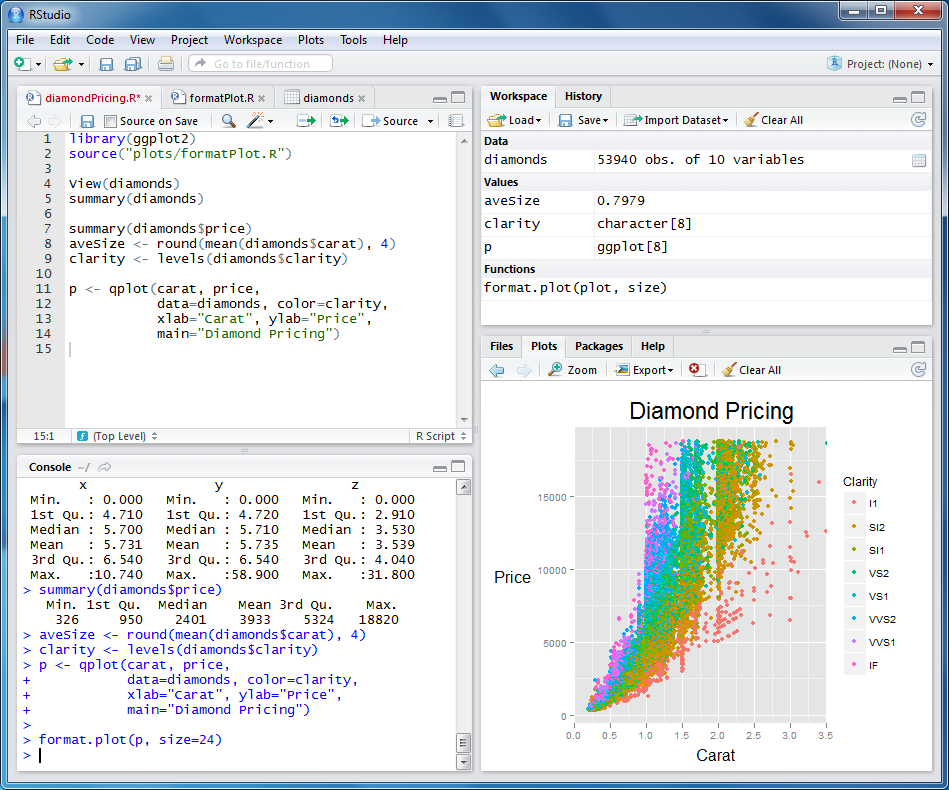 RStudio
To learn more about RStudio you can visit this post on RStudio Features
Installing R and RStudio
Note: R is installed before RStudio
The steps for installing R and RStudio include:
Step 1: Install R.
a. Download the R installer from this R CRAN Repository depending on your OS.
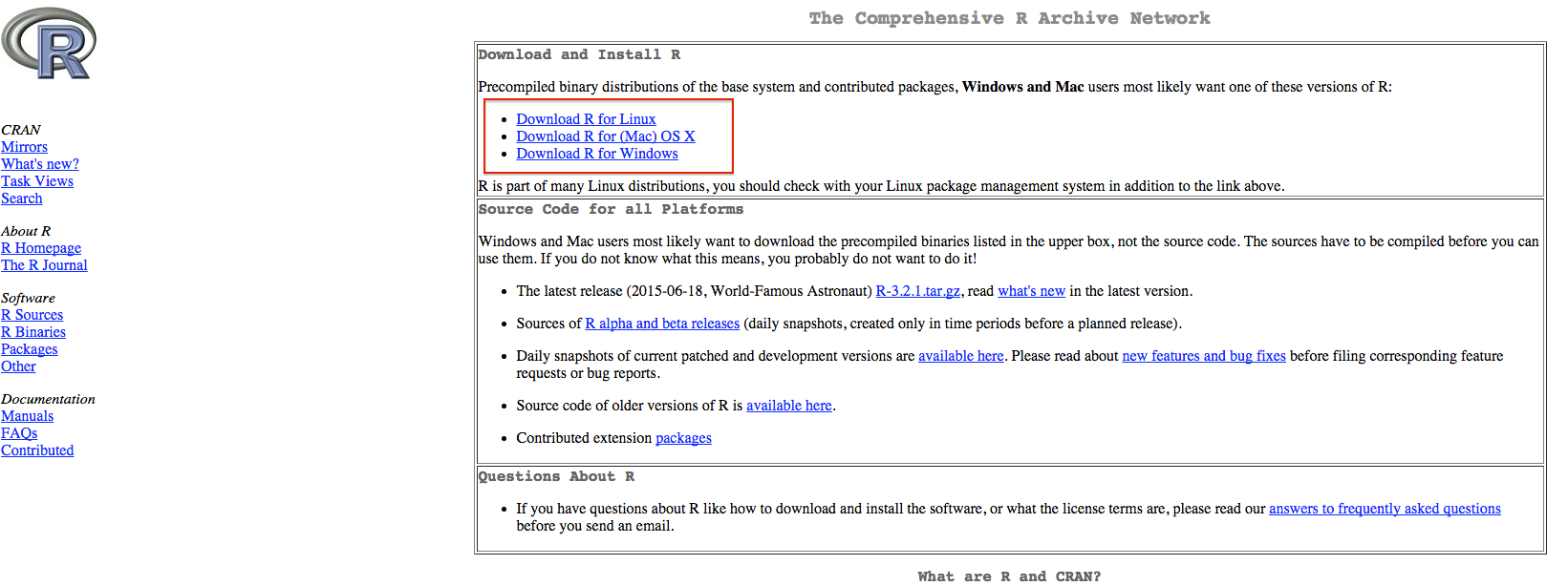
b. Run the installer. Default settings are fine.
Step 2: Install RStudio
a. Download RStudio from this RStudio Download Page depending on your OS:
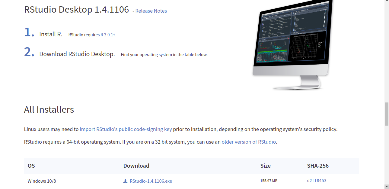
b. Run the RStudio installer
For Ubuntu 20.04 you can also follow this post
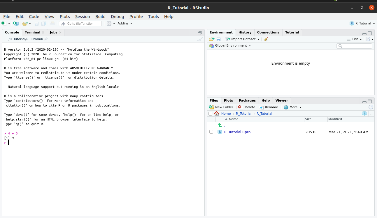
Step3 – Check that R and RStudio are working
a. Open RStudio. It should open a window that looks similar to image below.
b. In the left hand window, go to the console, by the ‘>’ sign, type ‘4+5’ (without the quotes) and hit enter. An output line reading ‘[1] 9’ should appear. This means that R and RStudio are working.
For more details on getting started with R, you can visit this R tutorial
R Basic Syntax
1. Declaring a variable
A variable provides us with named storage that our programs can manipulate. The variables can be assigned values using leftward, rightward or equal to operator.
> x <- 34          # Assignment using leftward operator.
> y -> 22          # Assignment using rightward operator
> z = 55           # Assignment using equal operator.
Note: comments in R are preceded by #
In a programming language, the information we store in variables could be an integer, character, floating-point, boolean, etc.
Programming languages like C, C++, and Java, variables are declared as data type; however, in Python and R, the variables are an object. Objects are a data structure having few attributes and methods which are applied to its attributes.
In R, a variable itself is not declared of any data type, rather it gets the data type of the R - object assigned to it. So R is called a dynamically typed language, which means that we can change a variable’s data type of the same variable again and again when using it in a program.
3. Data Structures and data types in R
Some data structures include: Vectors, Lists, Matrices, Arrays, Factors and Data Frames
Basic data types on which the R data structures are built include: Numeric, Integer, Character, Factor, and Logical.
You can check the data type of a using the class() function.
Numeric are numbers that have a decimal value
num = 1.2
class(num)                             # returns 'numeric'.
Integers are numbers that do not contain decimal
myint = 10
class(myint)                           # this returns 'integer'
A character can be a letter or a combination of letters enclosed by quotes is considered as a character data type by R. It can be alphabets or numbers.
mychar = "Hello There"
class(mychar)
print(mychar)                        # the print() function is used to print out the variables.
Factors are a data type that is used to refer to a qualitative relationship like colors, good & bad, course or movie ratings, etc. They are useful in statistical modeling.
fac = factor(c("good", "bad", "ugly","good", "bad", "ugly"))
print(fac)
This returns:
[1] good bad  ugly good bad  ugly
Levels: bad good ugly
Let's look at the various data structures we have mentioned:
1. Vectors
Vectors are an object which is used to store multiple information or values of the same data type.
A vector can be created with a function c(), which will combine all the elements and return a one-dimensional array.
marks = c(88,65,90,40,65)
class(marks)
# returns 'numeric'
To check the length of the vector, we will use the length() function which returns the number of elements contained in a variable.
length(marks)
# returns 5
We can access a specific element by its index
marks[4]
# returns 40
Note: In R indexing, the first element is given an index of 1
Slicing can also be applied:
marks[2:5]
# returns 65 90 40 65
Creating a character vector is similar to creating a numeric character:
char_vector = c("a", "b", "c")
print(char_vector)
[1] "a" "b" "c"
class(char_vector)
'character'
2. Matrix
A matrix is used to store information about the same data type. However, unlike vectors, matrices are capable of holding two-dimensional information inside it.
The syntax for defining a matrix is:
M = matrix(vector, nrow=r, ncol=c, byrow=FALSE, dimnames=list(char_vector_rownames, char_vector_colnames))
For example a 2 x 3 matrix
M = matrix( c('AI','ML','DL','Tensorflow','Pytorch','Keras'), nrow = 2, ncol = 3, byrow = TRUE)
print(M)
     [,1]         [,2]      [,3]
[1,] "AI"         "ML"      "DL"
[2,] "Tensorflow" "Pytorch" "Keras"
Let's use the slicing concept and fetch elements from a row and column.
M[1:2,1:2]
# The first dimension selects the first two rows while the second dimension will select the first two columns
     [,1]         [,2]
[1,] "AI"         "ML"
[2,] "Tensorflow" "Pytorch"
3. Data Frame
Unlike a matrix, Data frames are a more generalized form of a matrix. It contains data in a tabular fashion. The data in the data frame can be spread across various columns, having different data types.
DataFrame can be created using the data.frame() function.
DataFrame has been widely used in:
- reading comma-separated files (CSV), text files.
- machine learning problems, especially when dealing with numerical data in understanding the data, data wrangling, plotting and visualizing.
Let's create a dummy dataset and learn some data frame specific functions.
dataset <- data.frame(
   Person = c("Aditya", "Ayush","Akshay"),
   Age = c(26, 26, 27),
   Weight = c(81,85, 90),
   Height = c(6,5.8,6.2),
   Salary = c(50000, 80000, 100000)
)
print(dataset)
  Person Age Weight Height Salary
1 Aditya  26     81    6.0  5e+04
2  Ayush  26     85    5.8  8e+04
3 Akshay  27     90    6.2  1e+05
class(dataset)
'data.frame'
nrow(dataset)
# this will give you the number of rows that are there in the dataset dataframe
ncol(dataset)
# this will give you the number of columns that are there in the dataset dataframe
df1 = rbind(dataset, dataset)
# a row bind which will append the arguments in row fashion.
df1
This returns
  Person Age Weight Height Salary
1 Aditya  26     81    6.0  5e+04
2  Ayush  26     85    5.8  8e+04
3 Akshay  27     90    6.2  1e+05
4 Aditya  26     81    6.0  5e+04
5  Ayush  26     85    5.8  8e+04
6 Akshay  27     90    6.2  1e+05
df2 = cbind(df1, df1)
# a column bind which will append the arguments in column fashion.
df2
This returns
  Person Age Weight Height Salary Person Age Weight Height Salary
1 Aditya  26     81    6.0  5e+04 Aditya  26     81    6.0  5e+04
2  Ayush  26     85    5.8  8e+04  Ayush  26     85    5.8  8e+04
3 Akshay  27     90    6.2  1e+05 Akshay  27     90    6.2  1e+05
4 Aditya  26     81    6.0  5e+04 Aditya  26     81    6.0  5e+04
5  Ayush  26     85    5.8  8e+04  Ayush  26     85    5.8  8e+04
6 Akshay  27     90    6.2  1e+05 Akshay  27     90    6.2  1e+05
To look at the first few rows we use the head() function while to look at the last few rows we use the tail() function.
head(df1, 3)
# here only the first three rows will be printed
this returns:
  Person Age Weight Height Salary
1 Aditya  26     81    6.0  5e+04
2  Ayush  26     85    5.8  8e+04
3 Akshay  27     90    6.2  1e+05
tail(df1, 3)
# here only the last three rows will be printed
this returns:
  Person Age Weight Height Salary
4 Aditya  26     81    6.0  5e+04
5  Ayush  26     85    5.8  8e+04
6 Akshay  27     90    6.2  1e+05
str(dataset)
# this returns the individual class or data type information for each column.
'data.frame':    3 obs. of  5 variables:
 $ Person: Factor w/ 3 levels "Aditya","Akshay",..: 1 3 2
 $ Age   : num  26 26 27
 $ Weight: num  81 85 90
 $ Height: num  6 5.8 6.2
 $ Salary: num  5e+04 8e+04 1e+05
The summary() function, helps to understand the statistics of the data frame. As shown below, it divides your data into three quartiles, based on which you can get some intuition about the distribution of your data. It also shows if there are any missing values in your dataset.
summary(dataset)
Person       Age            Weight          Height        Salary
 Aditya:1   Min.   :26.00   Min.   :81.00   Min.   :5.8   Min.   : 50000
 Akshay:1   1st Qu.:26.00   1st Qu.:83.00   1st Qu.:5.9   1st Qu.: 65000
 Ayush :1   Median :26.00   Median :85.00   Median :6.0   Median : 80000
            Mean   :26.33   Mean   :85.33   Mean   :6.0   Mean   : 76667
            3rd Qu.:26.50   3rd Qu.:87.50   3rd Qu.:6.1   3rd Qu.: 90000
            Max.   :27.00   Max.   :90.00   Max.   :6.2   Max.   :100000
4. Lists
Unlike vectors, a list can contain elements of various data types. It can contain vectors, functions, matrices, and even another list inside it (nested-list).
You construct lists by using the list() function.
mylist = list(1:3, "a", c(TRUE, FALSE, TRUE), c(2.3, 5.9))
mylist
This returns:
[[1]]
[1] 1 2 3

[[2]]
[1] "a"

[[3]]
[1]  TRUE FALSE  TRUE

[[4]]
[1] 2.3 5.9
str(mylist)
This returns:
List of 4
 $ : int [1:3] 1 2 3
 $ : chr "a"
 $ : logi [1:3] TRUE FALSE TRUE
 $ : num [1:2] 2.3 5.9
If...else statement in R
Decision making is an important part of programming. This can be achieved in R programming using the conditional if...else statement.
If statement
The syntax of if statement is:
if (test_expression) {
statement
}
If the test_expression is TRUE, the statement gets executed. But if it’s FALSE, nothing happens.
for example:
x = 5
if (x  < 0){
print("The number is positive")
}

# The output is:
# [1] "Positive number"
If…else statement
The syntax of if…else statement is:
if (test_expression) {
statement1
} else {
statement2
}
The else part is optional and is only evaluated if test_expression is FALSE.
Note: else must be in the same line as the closing braces of the if statement.
If…else Ladder
The if…else ladder (if…else…if) statement allows you execute a block of code among more than 2 alternatives
The syntax of if…else statement is:
if ( test_expression1) {
statement1
} else if ( test_expression2) {
statement2
} else if ( test_expression3) {
statement3
} else {
statement4
}
Only one statement will get executed depending upon the test_expressions.
Example:
x = 0
if (x < 0) {
print("Negative number")
} else if (x > 0) {
print("Positive number")
} else
print("Zero")

# output is:
# [1] "Zero"
Loops
Loops are used in programming to repeat a specific block of code.
for loop in R
A for loop is used to iterate over a vector in R programming.
Syntax of for loop
for (val in sequence)
{
statement
}
Here, sequence is a vector and val takes on each of its value during the loop. In each iteration, the statement is evaluated.
Example:
a for loop to print out the elements in a vector
x = c(2,5,3,9)
count = 0
for (val in x) {
print(val)
}
This outputs:
[1] 2
[1] 5
[1] 3
[1] 9
Below is an example to count the number of even numbers in a vector.
x = c(2,5,3,9,8,11,6)
count = 0
for (val in x) {
if(val %% 2 == 0)  count = count+1
}
print(count)

# output is:
# [1] 3
Functions
A function is a set of statements organized together to perform a specific task.
R has a large number of in-built functions and the user can create their own functions.
1. In-built functions
So far we have used several pre-existing functions in R like the print(), data.frame(), list() functions among others.
Note: There are so many R in-built functions available so before defining your own,it would be better to see if what you need is already existing.
2. User-defined functions
Function Definition
An R function is created by using the keyword function. The basic syntax of an R function definition is as follows:
function_name = function(arg_1, arg_2, ...) {
   Function body
}
Function Components
The different parts of a function are:
Function Name − This is the actual name of the function. It is stored in R environment as an object with this name.
Arguments − An argument is a placeholder. When a function is invoked, you pass a value to the argument. Arguments are optional; that is, a function may contain no arguments. Also arguments can have default values.
Function Body − The function body contains a collection of statements that defines what the function does.
Return Value − The return value of a function is the last expression in the function body to be evaluated.
Example:
# Create a function to print squares of numbers in sequence.

new.function = function(a) {
   for(i in 1:a) {
      b = i^2
      print(b)
   }
}

# Call the function new.function supplying 6 as an argument.

new.function(6)
When we execute the above code, it produces the following result −
[1] 1
[1] 4
[1] 9
[1] 16
[1] 25
[1] 36
Object oriented programming in R
In R programming, OOPs (Object Oriented Programs) provides classes and objects as its key tools to reduce and manage the complexity of the program.
R is a functional language that uses concepts of OOPs.
We can think of class like a sketch of a car. It contains all the details about the model_name, model_no, engine etc. Based on these descriptions we select a car. Car is the object. Each car object has its own characteristics and features.
An object is also called an instance of a class and the process of creating this object is called instantiation.
OOPs has following features:
- Class
- Object
- Abstraction
- Encapsulation
- Polymorphism
- Inheritance
The two most important classes in R include:
- S3 Class
- S4 Class
1. S3 Class
S3 class does not have a predefined definition and ability to dispatch. In this class, the generic function makes a call to the method
It's syntax is:
variable_name = list(attribute1, attribute2, attribute3....attributeN)
Example: In the following code a Student class is defined. Appropriate class name is given having attributes student’s name and roll number. Then the object of student class is created and invoked.
# List creation with its attributes name and roll no.
a = list(name = "Adam", Roll_No = 15 )

# Defining a class "Student"
class(a) = "Student"

# Creation of object
a
Output:
$name
[1] "Adam"

$Roll_No
[1] 15

attr(, "class")
[1] "Student"
2. S4 Class
S4 class has a predefined definition. It contains functions for defining methods and generics. It makes multiple dispatches easy.
Syntax:
setClass("myclass", slots=list(name="character", Roll_No="numeric"))
Example:
# Function setClass() command is used to create S4 class containing list of slots.
setClass("Student", slots=list(name="character", Roll_No="numeric"))

# 'new' keyword used to create object of class 'Student'
a = new("Student", name="Adam", Roll_No=20)

# Calling object
a
Output:
Slot "name":
[1] "Adam"

Slot "Roll_No":
[1] 20
For more details on R OOP visit this R Object Oriented Programming post.
Installing packages
When you download R from the Comprehensive R Archive Network (CRAN), you get the "base" R system which comes with basic functionality;
One reason R is so useful is the large collection of packages that extend the basic functionality of R
R packages are developed and published by the larger R community
The primary location for obtaining R packages is CRAN
Packages can be installed with the install.packages() function in R
For example to install the rgdal package
install.packages("rgdal")
Note: The rgdal package provides bindings to the Geospatial Data Abstraction Library (GDAL) for reading, writing and converting between spatial formats.
To use the installed package, you have to import it using the library() function.
For instance after installing the rgdal package, to check the OGR Drivers installed:
library(rgdal)                         #import the rgdal package
ogrDrivers()$name
This returns:
##  [1] "AeronavFAA"     "ARCGEN"         "AVCBin"         "AVCE00"
##  [5] "BNA"            "CSV"            "DGN"            "DXF"
##  [9] "EDIGEO"         "ESRI Shapefile" "Geoconcept"     "GeoJSON"
## [13] "Geomedia"       "GeoRSS"         "GML"            "GMT"
## [17] "GPSBabel"       "GPSTrackMaker"  "GPX"            "HTF"
## [21] "Idrisi"         "KML"            "MapInfo File"   "Memory"
## [25] "MSSQLSpatial"   "ODBC"           "ODS"            "OpenAir"
## [29] "OpenFileGDB"    "PCIDSK"         "PDF"            "PDS"
## [33] "PGDump"         "PGeo"           "REC"            "S57"
## [37] "SDTS"           "SEGUKOOA"       "SEGY"           "SUA"
## [41] "SVG"            "SXF"            "TIGER"          "UK .NTF"
## [45] "VRT"            "Walk"           "WAsP"           "XLSX"
## [49] "XPlane"
Reference:


